



This talktorial introduces maximum common substructure (MCS) as a practical molecular-alignment tool for reaction informatics. We compare chemistry-aware RDKit MCS with explicit graph-level reasoning, then use the same idea for reaction rebalancing RDKit, 2026RDKit, 2026Phan et al., 2024.
Aim of this talktorial
Use MCS-based molecular alignment to compare molecules that differ by edits, substitutions, or missing components.
Interpret where RDKit MCS and graph-based MCS agree or differ.
Apply MCS reasoning to simple reaction rebalancing examples and connect it to SynRBL.
Learning outcomes
After completing this talktorial, you will be able to:
define maximum common substructure as a shared labeled subgraph,
compute and interpret MCS results with RDKit,
convert an MCS into an atom-level alignment between molecules,
explain why MCS results may be non-unique or sensitive to matching constraints,
use MCS-based alignment to reason about partial or noisy reactions, and
apply MCS ideas to simple reaction rebalancing examples.
0. Setup & Data
import warnings
import rdkit
from rdkit import Chem, RDLogger
import networkx as nx
import pandas as pd
import matplotlib.pyplot as plt
from pathlib import Path
from synedu.Utils.vis import draw_molecular_graph  # for visualization

# Keep the lesson output readable: RDKit narrates unmapped atoms on stderr and
# Matplotlib warns about layouts we set deliberately. Neither is a result.
RDLogger.DisableLog("rdApp.*")
warnings.filterwarnings("ignore", category=UserWarning)

print("RDKit version:", rdkit.__version__)
print("NetworkX version:", nx.__version__)

DATA_DIR = Path("data")
CSV_PATH = DATA_DIR / "molecules.csv"
df = pd.read_csv(CSV_PATH)
df['mol'] = df['smiles'].apply(Chem.MolFromSmiles)
display(df)
1. Maximum Common Substructure
The Maximum Common Substructure (MCS) RDKit, 2026Raymond & Willett, 2002 problem seeks the largest subgraph shared by two molecular graphs. It serves as a core alignment primitive for molecular similarity, substructure transfer, and as a common starting point for atom mapping.
1.1 Theory
Let
be labeled molecular graphs Diestel, 2017, where
A graph
is a common subgraph of (G) and (H) if there exist injective graph homomorphisms
that preserve adjacency and all labels.
An MCS is a common subgraph
that maximizes the number of vertices, i.e.
Practical notes.
MCSs are generally not unique.
Imposing chemical constraints (atom and bond types, aromaticity, ring membership, chirality) restricts the admissible homomorphisms and can change the resulting MCS.
Definition (Maximum Common Substructure / MCS).
Given two labeled graphs and , a common subgraph is a graph together with label-preserving injective homomorphisms and .
The maximum common subgraph (MCS) is a common subgraph of maximum cardinality (maximum common substructure by atoms) or maximum (by bonds).
Remark. MCS computation is NP-hard in general Raymond & Willett, 2002. RDKit’s FMCS search is exhaustive unless its timeout is reached; a cancelled search returns the best solution found so far. The compact NetworkX helper used below performs exact exponential backtracking for a maximum common induced vertex subgraph, which is a stricter problem than the general monomorphic definition above.
Definition (Normalized MCS size).
Given an MCS of two molecules, the normalized MCS size (Tanimoto-like) is:
This is 1 if the molecules are isomorphic and 0 if they share no atom.
1.2. RDKit MCS
In RDKit, the maximum common substructure (MCS) can be computed using
rdkit.Chem.rdFMCS RDKit, 2026.
RDKit MCS is commonly used for molecular alignment, reaction analysis, and as a basis for atom mapping.
from rdkit import Chem
from rdkit.Chem import rdFMCS, Draw


def rdkit_mcs(
    mols,
    timeout: int = 10,
    ringMatchesRingOnly: bool = True,
    maximizeBonds: bool = False,
    atomCompare=rdFMCS.AtomCompare.CompareElements,
    bondCompare=rdFMCS.BondCompare.CompareOrder,
):
    """
    Return the MCS SMARTS string and the rdFMCS result object.
    `mols` can be a list of RDKit Mol objects or SMILES strings.
    """
    mol_objs = [Chem.MolFromSmiles(s) if isinstance(s, str) else s for s in mols]
    if not mol_objs or any(mol is None for mol in mol_objs):
        raise ValueError("All MCS inputs must be valid molecules")
    res = rdFMCS.FindMCS(
        mol_objs,
        maximizeBonds=maximizeBonds,
        atomCompare=atomCompare,
        bondCompare=bondCompare,
        ringMatchesRingOnly=ringMatchesRingOnly,
        timeout=timeout,
    )
    return res.smartsString, res


def show_mcs_and_highlight(
    mols, smarts=None, show_all_matches=False, subimg_size=(300, 300)
):
    """
    Compute (or accept) MCS SMARTS, enumerate matches in each molecule,
    print a first-match atom-index mapping, and draw the molecules with
    highlighted MCS atoms.
    """
    # Accept SMILES or Mol
    mol_objs = [Chem.MolFromSmiles(s) if isinstance(s, str) else s for s in mols]
    if smarts is None:
        smarts, _ = rdkit_mcs(mol_objs)
    mcs_query = Chem.MolFromSmarts(smarts)

    # find matches
    matches = [tuple(m.GetSubstructMatches(mcs_query)) for m in mol_objs]
    match_counts = [len(ms) for ms in matches]

    print("MCS SMARTS:", smarts)
    for i, (m, cnt) in enumerate(zip(mol_objs, match_counts)):
        print(f"Mol {i+1}: {m.GetNumAtoms()} atoms, MCS matches: {cnt}")

    # If no matches found (shouldn't happen), return
    if any(cnt == 0 for cnt in match_counts):
        print("Warning: no MCS embedding found in one or more molecules.")
        return

    # Show mapping for the *first* embedding in each molecule
    first_matches = [ms[0] for ms in matches]
    mapping = (
        list(zip(first_matches[0], first_matches[1]))
        if len(first_matches) >= 2
        else None
    )
    if mapping:
        print("\nAtom mapping (mol1_atom -> mol2_atom) for first embeddings:")
        print(mapping)

    # Prepare highlight lists: choose which embedding to highlight for each molecule
    if show_all_matches:
        # create list-of-lists where we highlight all embeddings (flatten duplicates visually)
        hl_lists = [list(set(sum([list(t) for t in ms], []))) for ms in matches]
    else:
        hl_lists = [list(ms[0]) for ms in matches]

    # Legend labels
    legends = [
        mol.GetProp("_Name") if mol.HasProp("_Name") else f"Mol {i+1}"
        for i, mol in enumerate(mol_objs)
    ]

    # Draw side-by-side with highlighted atoms
    img = Draw.MolsToGridImage(
        mol_objs,
        molsPerRow=len(mol_objs),
        subImgSize=subimg_size,
        legends=legends,
        highlightAtomLists=hl_lists,
    )
    display(img)  # in a Jupyter notebook; returns PIL Image otherwise


m1 = Chem.MolFromSmiles("Oc1ccccc1")
m1.SetProp("_Name", "phenol")
m2 = Chem.MolFromSmiles("Cc1ccccc1")
m2.SetProp("_Name", "toluene")

smarts, res = rdkit_mcs([m1, m2])
show_mcs_and_highlight(
    [m1, m2], smarts=smarts, show_all_matches=False, subimg_size=(400, 400)
)
Stored in synedu.Utils — the MCS helpers are deposited for later reaction-alignment tasks:
from synedu.Utils.mcs import rdkit_mcs, nx_mcs, mcs_size, mcs_class, map_edgesLater notebooks can reuse these functions without carrying the teaching implementation forward.
Q1 — Compute the MCS between ethanol and another molecule
Use RDKit MCS to compute the maximum common substructure between ethanol and each molecule in the table, and record the size of the MCS.
This exercise shows how RDKit abstracts chemical similarity beyond strict subgraph containment.
Step-by-step tasks
Select ethanol as the reference molecule
Use the RDKit molecule corresponding to ethanol (row 0).Compute RDKit MCS
For each molecule, compute the MCS SMARTS between ethanol and the molecule usingrdkit_mcs.Convert SMARTS to a molecule
Turn the SMARTS into an RDKit query molecule.Measure MCS size
Record the number of atoms in the MCS (or0if no MCS is found).Store the result
Add a columnmcs_size_ethanol_rdkit.
Solution
ethanol_mol = df.loc[0, "mol"]

def rdkit_mcs_size_with_ethanol(mol):
    smarts, _ = rdkit_mcs([ethanol_mol, mol])
    if not smarts:
        return 0
    mcs_mol = Chem.MolFromSmarts(smarts)
    if mcs_mol is None:
        return 0
    return mcs_mol.GetNumAtoms()

df["mcs_size_ethanol_rdkit"] = df["mol"].apply(rdkit_mcs_size_with_ethanol)
df
1.3. NetworkX MCS
from __future__ import annotations

from itertools import combinations
from typing import Dict, Set, Tuple

import networkx as nx
from networkx.algorithms import isomorphism as iso
from rdkit import Chem


def nx_mcs(
    G: nx.Graph,
    H: nx.Graph,
    *,
    node_match,
    edge_match,
) -> tuple[nx.Graph, Dict[int, int]]:
    """
    Return one maximum common induced subgraph SG of G, plus a node mapping SG->H.
    Exponential; for teaching only.
    """
    nodes = list(G.nodes())
    for k in range(len(nodes), 0, -1):
        for subset in combinations(nodes, k):
            SG = G.subgraph(subset).copy()

            GM = iso.GraphMatcher(H, SG, node_match=node_match, edge_match=edge_match)
            if GM.subgraph_is_isomorphic():
                # GraphMatcher mapping is H -> SG; invert to get SG -> H
                h_to_sg = next(GM.subgraph_isomorphisms_iter())
                sg_to_h = {sg: h for h, sg in h_to_sg.items()}
                return SG, sg_to_h

    return nx.Graph(), {}


def _map_edges(
    SG: nx.Graph, sg_to_h: Dict[int, int], H: nx.Graph
) -> Set[Tuple[int, int]]:
    """Map SG edges into H using sg_to_h; returns undirected edge tuples."""
    out: Set[Tuple[int, int]] = set()
    for u, v in SG.edges():
        hu, hv = sg_to_h[u], sg_to_h[v]
        if H.has_edge(hu, hv):
            out.add((hu, hv))
    return out
from synedu.Utils import mol_to_graph, node_match, edge_match, draw_molecular_graph
import matplotlib.pyplot as plt
m1 = Chem.MolFromSmiles("Oc1ccccc1") # phenol
m2 = Chem.MolFromSmiles("Cc1ccccc1") # toluene
# Convert to labeled NetworkX graphs (nodes must be atom indices)
m1_g = mol_to_graph(m1)
m2_g = mol_to_graph(m2)
# Compute NX MCS + one embedding (SG -> m2_g mapping)
SG, sg_to_h = nx_mcs(m1_g, m2_g, node_match=node_match, edge_match=edge_match)
print("MCS nodes:", SG.number_of_nodes(), "MCS edges:", SG.number_of_edges())
print("One SG->H mapping (first):", sg_to_h)
# Highlight sets
hl_m1_nodes = set(SG.nodes())
hl_m1_edges = set(SG.edges())
hl_m2_nodes = {sg_to_h[n] for n in SG.nodes()}
hl_m2_edges = _map_edges(SG, sg_to_h, m2_g)
fig, axes = plt.subplots(1, 2, figsize=(10, 4))
draw_molecular_graph(
m1_g,
ax=axes[0],
include_mol=False,
highlight_nodes=hl_m1_nodes,
highlight_edges=hl_m1_edges,
)
axes[0].set_title("Phenol", fontsize=20, weight='bold')
draw_molecular_graph(
m2_g,
ax=axes[1],
include_mol=False,
highlight_nodes=hl_m2_nodes,
highlight_edges=hl_m2_edges,
)
axes[1].set_title("Toluene", fontsize=20, weight='bold')
plt.tight_layout()
plt.show()MCS alignment gallery
Each row shows a molecule pair. The highlighted (orange) atoms and bonds form the maximum common substructure. Larger MCS → more shared scaffold; smaller MCS → structurally divergent molecules despite similar element composition.
Source
from rdkit import Chem
from rdkit.Chem import rdFMCS
import matplotlib.pyplot as plt
from synedu.Utils import mol_to_graph, draw_molecular_graph

_MCS_PAIRS = [
    ("phenol", "Oc1ccccc1", "toluene", "Cc1ccccc1"),
    ("ethanol", "CCO", "propanol", "CCCO"),
    ("acetone", "CC(C)=O", "butanone", "CCC(C)=O"),
    ("naphthalene", "c1ccc2ccccc2c1", "indene", "C1=CC2=CC=CC=C2C1"),
]

fig, axes = plt.subplots(len(_MCS_PAIRS), 2, figsize=(10, 4 * len(_MCS_PAIRS)))
fig.suptitle(
    "MCS alignment — highlighted region is the maximum common substructure",
    fontsize=11,
    fontweight="bold",
)

for row, (n1, smi1, n2, smi2) in enumerate(_MCS_PAIRS):
    m1 = Chem.MolFromSmiles(smi1)
    m2 = Chem.MolFromSmiles(smi2)
    g1 = mol_to_graph(m1)
    g2 = mol_to_graph(m2)

    smarts, _ = rdkit_mcs([m1, m2])
    mcs_q = Chem.MolFromSmarts(smarts) if smarts else None

    match1 = m1.GetSubstructMatch(mcs_q) if mcs_q else ()
    match2 = m2.GetSubstructMatch(mcs_q) if mcs_q else ()

    hl1 = set(match1)
    hl1_e = {(u, v) for u, v in g1.edges() if u in hl1 and v in hl1}
    hl2 = set(match2)
    hl2_e = {(u, v) for u, v in g2.edges() if u in hl2 and v in hl2}

    ax1, ax2 = axes[row, 0], axes[row, 1]
    draw_molecular_graph(
        g1,
        ax=ax1,
        include_mol=False,
        highlight_nodes=hl1,
        highlight_edges=hl1_e,
        highlight_color="#FF7F0E",
    )
    ax1.set_title(f"{n1}  [{len(hl1)} MCS atoms]", fontsize=10, weight="bold")

    draw_molecular_graph(
        g2,
        ax=ax2,
        include_mol=False,
        highlight_nodes=hl2,
        highlight_edges=hl2_e,
        highlight_color="#FF7F0E",
    )
    ax2.set_title(f"{n2}  [{len(hl2)} MCS atoms]", fontsize=10, weight="bold")

plt.tight_layout()
plt.show()
Q2 — Compute the MCS between ethanol and another molecule
Compute the MCS between ethanol and each molecule in the table using the NetworkX-based MCS implementation, and record the size of the resulting common subgraph.
This exercise emphasizes a strict graph-theoretic view of MCS, in contrast to the chemistry-aware RDKit approach in Q1.
Step-by-step tasks
Select ethanol as the reference graph
Use the NetworkX graph corresponding to ethanol (row 0).Compute NetworkX MCS
For each molecule graph, compute an MCS usingnx_mcs.Measure MCS size
Record the number of nodes (atoms) in the resulting MCS graph.Store the result
Add a new columnmcs_size_ethanol_nxto the dataframe.
Solution
# Reference graph: ethanol
df['graph'] = df['mol'].apply(mol_to_graph)
ethanol_G = df.loc[0, "graph"]

def nx_mcs_size_with_ethanol(host_G):
    S, _ = nx_mcs(
        ethanol_G,
        host_G,
        node_match=node_match,
        edge_match=edge_match,
    )
    if S is None:
        return 0
    return S.number_of_nodes()

# Add NetworkX MCS size column
df["mcs_size_ethanol_nx"] = df["graph"].apply(nx_mcs_size_with_ethanol)
The following comparison isolates cases where the RDKit and NetworkX MCS definitions disagree.
df[df['mcs_size_ethanol_rdkit'] != df['mcs_size_ethanol_nx']]Most discrepancies originate from ring systems. RDKit MCS is chemistry-first, enforcing ring–chain consistency, whereas NetworkX MCS is graph-first and performs purely topological matching. With RingMatchesRingOnly=True, RDKit allows atom matches only when both the pattern and host atoms belong to rings, preventing acyclic–ring correspondences. Consequently, cyclic hydrocarbons yield zero MCS with ethanol under RDKit but non-zero matches under unconstrained graph matching.
MCS size vs Tanimoto similarity
Tanimoto similarity (fingerprint-based) and MCS size (graph-based) both measure molecular overlap, but they are not equivalent Raymond & Willett, 2002. The scatter plot below samples molecules from the dataset and compares both metrics against ethanol. Ring-containing molecules can have high graph MCS under RDKit’s chemistry-aware matcher yet low Tanimoto — or vice versa.
Source
import numpy as np
import pandas as pd
import matplotlib.pyplot as plt
import matplotlib.colors as mcolors

from rdkit import Chem, DataStructs
from rdkit.Chem import rdFMCS
from rdkit.Chem import rdFingerprintGenerator

_ref_smi = "CCO"  # ethanol
_n_sample = 150
_random_state = 7
_mcs_timeout = 3

_fp_radius = 2
_fp_size = 1024


_ref_mol = Chem.MolFromSmiles(_ref_smi)
_ref_atoms = _ref_mol.GetNumAtoms()

_morgan_gen = rdFingerprintGenerator.GetMorganGenerator(
    radius=_fp_radius, fpSize=_fp_size
)

_ref_fp = _morgan_gen.GetFingerprint(_ref_mol)


def _safe_mol_from_smiles(smi):
    if not isinstance(smi, str) or not smi.strip():
        return None
    try:
        return Chem.MolFromSmiles(smi)
    except Exception:
        return None


def _mcs_size(mol_a, mol_b, timeout=3):
    """
    Return MCS atom count.

    This first tries your existing rdkit_mcs(...) wrapper if available.
    If not available, it falls back to RDKit's rdFMCS.FindMCS.
    """
    try:
        _smarts, _ = rdkit_mcs([mol_a, mol_b], timeout=timeout)
        _q = Chem.MolFromSmarts(_smarts) if _smarts else None
        return _q.GetNumAtoms() if _q is not None else 0

    except NameError:
        try:
            res = rdFMCS.FindMCS(
                [mol_a, mol_b],
                timeout=timeout,
                ringMatchesRingOnly=True,
                completeRingsOnly=True,
                matchValences=True,
            )
            if res.canceled or not res.smartsString:
                return 0
            _q = Chem.MolFromSmarts(res.smartsString)
            return _q.GetNumAtoms() if _q is not None else 0
        except Exception:
            return 0

    except Exception:
        return 0


def _mcs_class(mcs_atoms, ref_atoms):
    if mcs_atoms == ref_atoms:
        return "full reference MCS"
    elif mcs_atoms == ref_atoms - 1:
        return "large partial MCS"
    elif mcs_atoms == 1:
        return "single-atom MCS"
    else:
        return "weak/no MCS"


_sample_smis = (
    df["smiles"]
    .dropna()
    .drop_duplicates()
    .sample(
        n=min(_n_sample, df["smiles"].dropna().drop_duplicates().shape[0]),
        random_state=_random_state,
    )
    .tolist()
)

_records = []

for _smi in _sample_smis:
    _mol = _safe_mol_from_smiles(_smi)
    if _mol is None:
        continue

    _fp = _morgan_gen.GetFingerprint(_mol)
    _tan = DataStructs.TanimotoSimilarity(_ref_fp, _fp)

    _sz = _mcs_size(_ref_mol, _mol, timeout=_mcs_timeout)

    _mcs_cov = _sz / _ref_atoms
    _gap = _mcs_cov - _tan

    _records.append(
        {
            "smiles": _smi,
            "canonical_smiles": Chem.MolToSmiles(_mol),
            "tanimoto": _tan,
            "mcs_atoms": _sz,
            "mcs_ref_coverage": _mcs_cov,
            "gap_mcs_minus_fp": _gap,
            "heavy_atoms": _mol.GetNumHeavyAtoms(),
            "class": _mcs_class(_sz, _ref_atoms),
        }
    )

_pts = pd.DataFrame(_records)


if _pts.empty:
    print("No valid molecules found.")

else:
    rng = np.random.default_rng(_random_state)

    # Small vertical jitter reveals overlapping points while preserving integer MCS bands
    _pts["mcs_atoms_jitter"] = _pts["mcs_atoms"] + rng.normal(0, 0.035, size=len(_pts))

    fig = plt.figure(figsize=(10.6, 5.8))

    gs = fig.add_gridspec(
        1,
        2,
        width_ratios=[3.25, 1.15],
        wspace=0.30,
    )

    ax = fig.add_subplot(gs[0, 0])
    ax_box = fig.add_subplot(gs[0, 1])

    _gap = _pts["gap_mcs_minus_fp"]
    _lim = max(abs(_gap.min()), abs(_gap.max()), 1e-6)

    _norm = mcolors.TwoSlopeNorm(
        vmin=-_lim,
        vcenter=0,
        vmax=_lim,
    )

    sc = ax.scatter(
        _pts["tanimoto"],
        _pts["mcs_atoms_jitter"],
        c=_pts["gap_mcs_minus_fp"],
        cmap="coolwarm",
        norm=_norm,
        s=35 + 2.7 * _pts["heavy_atoms"],
        alpha=0.72,
        edgecolors="white",
        linewidths=0.45,
    )

    _xline = np.linspace(0, 1, 200)

    ax.plot(
        _xline,
        _xline * _ref_atoms,
        linestyle="--",
        linewidth=1.2,
        color="black",
        alpha=0.55,
    )

    # Integer MCS guide lines
    for y in range(_ref_atoms + 1):
        ax.axhline(
            y,
            linestyle=":",
            linewidth=0.9,
            color="gray",
            alpha=0.35,
        )

    # Highlight molecules with full ethanol-sized MCS
    full = _pts[_pts["mcs_atoms"] == _ref_atoms]

    ax.scatter(
        full["tanimoto"],
        full["mcs_atoms_jitter"],
        facecolors="none",
        edgecolors="black",
        s=95,
        linewidths=0.8,
        alpha=0.75,
    )

    cbar = plt.colorbar(sc, ax=ax, pad=0.02)

    cbar.set_label(
        "MCS coverage − Tanimoto",
        fontsize=8.5,
    )

    ax.set_xlabel(
        f"Tanimoto similarity  (Morgan r={_fp_radius}, {_fp_size} bits)",
        fontsize=10,
    )

    ax.set_ylabel(
        "MCS size shared with ethanol  (atoms)",
        fontsize=10,
    )

    ax.set_title(
        "MCS vs Tanimoto — ethanol reference",
        fontsize=11,
        fontweight="bold",
    )

    ax.set_xlim(-0.02, 1.02)
    ax.set_ylim(-0.25, _ref_atoms + 0.35)
    ax.set_yticks(range(_ref_atoms + 1))

    ax.grid(alpha=0.16)
    ax.spines[["top", "right"]].set_visible(False)

    grouped = [
        _pts.loc[_pts["mcs_atoms"] == i, "tanimoto"].values
        for i in range(_ref_atoms + 1)
    ]

    ax_box.boxplot(
        grouped,
        positions=list(range(_ref_atoms + 1)),
        widths=0.55,
        showfliers=False,
        patch_artist=True,
        boxprops=dict(
            facecolor="white",
            edgecolor="black",
            linewidth=0.9,
        ),
        medianprops=dict(
            color="black",
            linewidth=1.2,
        ),
        whiskerprops=dict(
            color="black",
            linewidth=0.8,
        ),
        capprops=dict(
            color="black",
            linewidth=0.8,
        ),
    )

    for i in range(_ref_atoms + 1):
        vals = _pts.loc[_pts["mcs_atoms"] == i, "tanimoto"].values
        if len(vals) == 0:
            continue

        xj = rng.normal(i, 0.045, size=len(vals))

        ax_box.scatter(
            xj,
            vals,
            s=18,
            alpha=0.5,
            edgecolors="none",
        )

    ax_box.set_xlabel("MCS atoms", fontsize=9)
    ax_box.set_ylabel("Tanimoto distribution", fontsize=9)

    ax_box.set_title(
        "Tanimoto by MCS",
        fontsize=9,
        fontweight="bold",
    )

    ax_box.set_xticks(range(_ref_atoms + 1))
    ax_box.set_ylim(-0.02, 1.02)

    ax_box.grid(axis="y", alpha=0.18)
    ax_box.spines[["top", "right"]].set_visible(False)

    plt.tight_layout()
    plt.show()


if not _pts.empty:
    insight_table = _pts.sort_values("gap_mcs_minus_fp", ascending=False)[
        [
            "canonical_smiles",
            "tanimoto",
            "mcs_atoms",
            "mcs_ref_coverage",
            "gap_mcs_minus_fp",
            "heavy_atoms",
            "class",
        ]
    ].reset_index(drop=True)

    display(insight_table.head(10))
2. Rule-based reaction rebalancing
This section follows the idea of Reaction rebalancing: a novel approach to curating reaction databases Phan et al., 2024.
2.1 Reaction decomposition
Given a reaction SMILES
define the reactant and product multisets
2.2 Formula representation
Let be the set of chemical elements. Each molecule is represented by its augmented conservation vector
where contains the element counts and is the net formal charge. Total conserved quantities are
2.3 Imbalance detection
Define the imbalance vector
The reaction is atom- and charge-balanced if and only if
. Atom counts alone cannot distinguish, for example,
[Na+]>>[Na-].
2.4 Auxiliary-species imputation
Let be a library of auxiliary species (e.g. ) with vectors . Let denote how many copies of are added to the reactant and product sides, respectively. We seek coefficients satisfying
This integer equation handles element counts and charge together. In a one-sided repair, either all or all are constrained to zero.
2.5 Reaction update
If an admissible solution exists, rebalance the reaction by adding the corresponding auxiliary species:
where denotes multiset union. In reaction SMILES, this corresponds
to appending each auxiliary component to the selected side (for example, O
for ). Chemical admissibility constraints are still required:
the conservation equation alone does not establish that a proposed repair is
mechanistically or experimentally appropriate.
Rebalancing workflow
The pipeline below converts an imbalanced reaction SMILES into a balanced one. Conservation analysis routes each record by reaction class: rule-library search repairs formula-level gaps (small inorganic species), while MCS alignment recovers missing carbon fragments. Every route ends at the same validation gate, and a record that cannot be balanced admissibly is returned unchanged.
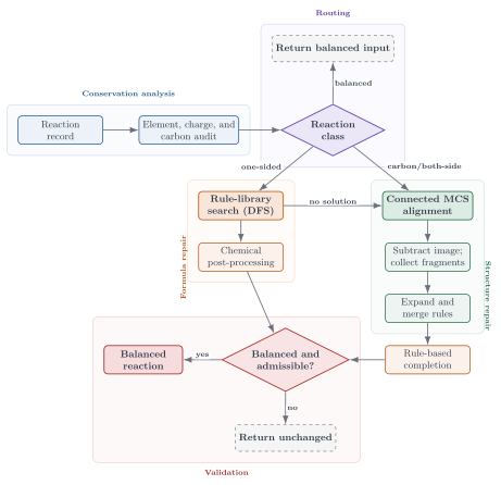
Figure 1. The SynRBL rebalancing pipeline. Blue: conservation analysis. Purple: routing by reaction class. Orange: formula repair via rule-library search. Green: structure repair via connected MCS alignment. Red: validation, which either emits a balanced reaction or returns the record unchanged.
The MCS branch is the interesting one for this talktorial. Aligning the two sides exposes exactly which fragment is unaccounted for, and the missing substructure is then expanded and merged back into the deficient side.
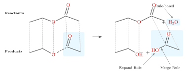
Figure 2. MCS-guided rebalancing. Dashed guides mark the atom correspondence recovered by the maximum common substructure; the shaded region is the unmatched fragment. Rule-based imputation supplies the missing water, while the expand and merge rules reconstruct the acid fragment on the product side.
Now consider the following simple reaction. By comparing the total molecular formulas of the reactant and product sides, we can immediately detect a missing water molecule on the product side.
from synedu.Utils import draw_rxn_graph

fig = draw_rxn_graph(
    'CCO>>C=C',
    title="Elimination",
    highlight_changes=True,
    label_mode="hetero",
    show_indices=False,
    aromatic_style="circle",
    show_legend=False,
)
To automate this imputation, we introduce a small set of utility functions for parsing reactions, computing formula imbalances, and resolving them using predefined auxiliary species.
from __future__ import annotations

from collections import Counter
from typing import Tuple

from rdkit import Chem


# Reaction decomposition


def parse_reaction_smiles(rsmi: str) -> Tuple[list[Chem.Mol], list[Chem.Mol]]:
    """
    Parse a reaction SMILES into reactant and product molecule lists.

    Parameters
    ----------
    rsmi : str
        Reaction SMILES, e.g. "CCO.O>>CC=O"

    Returns
    -------
    reactants : list[Chem.Mol]
    products  : list[Chem.Mol]
    """
    try:
        lhs, rhs = rsmi.split(">>")
    except ValueError:
        raise ValueError("Reaction SMILES must contain '>>'")

    reactants = [Chem.MolFromSmiles(s) for s in lhs.split(".") if s]
    products = [Chem.MolFromSmiles(s) for s in rhs.split(".") if s]

    if any(m is None for m in reactants + products):
        raise ValueError("Invalid molecule in reaction SMILES")

    return reactants, products


# Formula representation


def molecular_formula(mol: Chem.Mol) -> Counter[str]:
    """
    Compute element counts and net formal charge for one molecule.

    Returns
    -------
    Counter[str]
        Mapping element symbol -> atom count
    """
    mol = Chem.AddHs(mol)

    formula = Counter()
    for atom in mol.GetAtoms():
        formula[atom.GetSymbol()] += 1
        formula["__charge__"] += int(atom.GetFormalCharge())
    if formula["__charge__"] == 0:
        del formula["__charge__"]
    return formula


def total_formula(mols: list[Chem.Mol]) -> Counter[str]:
    """
    Compute total formula Φ = sum φ(M) over a list of molecules.
    """
    total = Counter()
    for m in mols:
        for key, value in molecular_formula(m).items():
            total[key] += value
    if total["__charge__"] == 0:
        del total["__charge__"]
    return total


# Imbalance detection

from collections import Counter
from typing import Literal, Tuple


def signed_difference(a: Counter[str], b: Counter[str]) -> Counter[str]:
    """
    Compute signed element-wise difference a - b
    without dropping negative values.
    """
    delta = Counter()
    for elem in set(a) | set(b):
        v = a.get(elem, 0) - b.get(elem, 0)
        if v != 0:
            delta[elem] = v
    return delta


def reaction_imbalance(
    rsmi: str,
) -> Tuple[
    Counter[str],
    Literal[
        "balanced",
        "missing_in_products",
        "missing_in_reactants",
        "missing_in_both_sides",
    ],
]:
    """
    Compute the reaction imbalance vector Δ = Φ_R − Φ_P
    and classify where material is missing.

    Returns
    -------
    delta : Counter[str]
        Element-wise imbalance (positive = excess on reactant side)
    status : str
        One of:
        - 'balanced'
        - 'missing_in_products'
        - 'missing_in_reactants'
        - 'missing_in_both_sides'
    """
    reactants, products = parse_reaction_smiles(rsmi)

    phi_R = total_formula(reactants)
    phi_P = total_formula(products)
    delta = signed_difference(phi_R, phi_P)

    if not delta:
        return delta, "balanced"

    has_pos = any(v > 0 for v in delta.values())
    has_neg = any(v < 0 for v in delta.values())

    if has_pos and not has_neg:
        status = "missing_in_products"
    elif has_neg and not has_pos:
        status = "missing_in_reactants"
    else:
        status = "missing_in_both_sides"

    return delta, status
Stored in synedu.Utils — reaction-balance helpers are now packaged for later curation and rule-extraction steps:
from synedu.Utils.reaction import parse_reaction_smiles, reaction_imbalanceThis keeps the formula-balance convention consistent across later tasks.
rsmi = 'CCO>>C=C'
delta, status = reaction_imbalance(rsmi)
print(delta, status)
from collections import Counter
from typing import Dict, Optional
AUX_LIBRARY: Dict[str, Counter[str]] = {
"O": Counter({"H": 2, "O": 1}), # H2O
"[H+]": Counter({"H": 1}),
"[OH-]": Counter({"H": 1, "O": 1}),
}Q3 — Auxiliary imputation feasibility
You are given an element-wise imbalance vector
and an auxiliary species with molecular formula
The goal is to decide whether the imbalance can be resolved by adding copies of , i.e.
Hint:
Think element-wise.
If such a exists, then for every element ,
the ratio must be:
an integer,
the same for all elements,
and strictly positive.
Also ensure that no extra elements remain unexplained.
Solution
from collections import Counter
from typing import Optional


def can_impute_with_aux(
    delta: Counter[str],
    aux_formula: Counter[str],
) -> Optional[int]:
    """
    Check whether Δ can be written as c · φ(A).
    """
    if not delta:
        return 0

    ratios = []

    for elem, count in aux_formula.items():
        if elem not in delta:
            return None
        if delta[elem] % count != 0:
            return None
        ratios.append(delta[elem] // count)

    if not ratios or len(set(ratios)) != 1:
        return None

    c = ratios[0]
    if c <= 0:
        return None

    remainder = delta - Counter({k: c * v for k, v in aux_formula.items()})
    if remainder:
        return None

    return c
def impute_rsmi_rule(
rsmi: str,
delta: Counter[str],
status: str,
library: Dict[str, Counter[str]] = AUX_LIBRARY,
) -> Optional[str]:
if status == "balanced":
return rsmi
if status == "missing_in_both_sides":
return None
lhs, rhs = rsmi.split(">>")
# decide direction
if status == "missing_in_products":
target_delta = delta
side = "products"
elif status == "missing_in_reactants":
target_delta = -delta
side = "reactants"
else:
return None
# try library
for aux_smiles, formula in library.items():
c = can_impute_with_aux(target_delta, formula)
if c is None:
continue
aux_block = ".".join([aux_smiles] * c)
if side == "products":
rhs = rhs + "." + aux_block if rhs else aux_block
else:
lhs = lhs + "." + aux_block if lhs else aux_block
return f"{lhs}>>{rhs}"
return None
def can_impute_with_aux(
delta: Counter[str],
aux_formula: Counter[str],
) -> Optional[int]:
"""
Check whether Δ can be written as c · φ(A).
"""
if not delta:
return 0
ratios = []
for elem, count in aux_formula.items():
if elem not in delta:
return None
if delta[elem] % count != 0:
return None
ratios.append(delta[elem] // count)
if not ratios or len(set(ratios)) != 1:
return None
c = ratios[0]
if c <= 0:
return None
remainder = delta - Counter({k: c * v for k, v in aux_formula.items()})
if remainder:
return None
return cStored in synedu.Utils — auxiliary-species imputation is available as a reusable utility:
from synedu.Utils.reaction import AUX_LIBRARY, can_impute_with_aux, impute_rsmi_ruleLater notebooks can focus on when to impute, rather than redefining the same bookkeeping.
Now try with the above example
delta, status = reaction_imbalance(rsmi)
rsmi_balanced = impute_rsmi_rule(rsmi, delta, status, library=AUX_LIBRARY)

print(rsmi_balanced)
if rsmi_balanced:
    fig = draw_rxn_graph(
        rsmi_balanced,
        title="E1 example",
        highlight_changes=True,
        label_mode="hetero",
        show_indices=False,
        aromatic_style="circle",
        show_legend=False,
    )
Before / after rebalancing
Imbalanced reactions are missing one or more species. The gallery below shows each reaction before and after library-based imputation — atoms and bonds are unchanged; only the missing auxiliary species (water, HCl) are appended to the correct side.
Source
from collections import Counter
from synedu.Utils.rxn_vis import draw_rxn_graph
import matplotlib.pyplot as plt

_AUX_EXT = {
    "O": Counter({"H": 2, "O": 1}),
    "[H+]": Counter({"H": 1}),
    "[OH-]": Counter({"H": 1, "O": 1}),
    "Cl": Counter({"H": 1, "Cl": 1}),
}

_EXAMPLES = [
    ("CCO>>C=C", "E1 elimination"),
    ("CC(C)O.Cl>>CC(C)Cl", "Nucleophilic substitution"),
]

for rsmi_ex, title in _EXAMPLES:
    delta_ex, status_ex = reaction_imbalance(rsmi_ex)
    rsmi_bal_ex = (
        impute_rsmi_rule(rsmi_ex, delta_ex, status_ex, library=_AUX_EXT) or rsmi_ex
    )

    print(f"\n{title}")
    print("Before (imbalanced):")
    draw_rxn_graph(rsmi_ex, title=title, highlight_changes=False, show_legend=False)
    plt.show()

    print("After (rebalanced):")
    draw_rxn_graph(
        rsmi_bal_ex,
        title=f"{title} — rebalanced",
        highlight_changes=False,
        show_legend=False,
    )
    plt.show()

    print("-" * 48)
Q4 — Rebalance some reactions
Extend the auxiliary-species library and use it to rebalance these reactions:
CC(C)O>>CC(C)Cl.O
CC(C)Cl>>CC(C)N.Cl
CC(=O)O>>CC(=O)OC.O
Solution idea
add common auxiliary species such as water, hydrochloric acid, ammonia, hydroxide, and methanol to the library. For each reaction, compute the imbalance with reaction_imbalance, call impute_rsmi, and keep the balanced reaction when imputation succeeds.
3. MCS-based reaction rebalancing
For non-carbon compounds, missing species can often be imputed from a finite library. In contrast, for carbon-containing compounds, the space of possible structures grows exponentially, making library-based enumeration impractical at scale.
Instead, we use reaction alignment to identify missing structural motifs via MCS and apply rule-based reasoning to complete and rebalance reactions.
In this section, we directly use functionality from SynKit Phan et al., 2025
(pip install synkit) and explore an established tool for reaction rebalancing,
SynRBL Phan et al., 2024 (pip install synrbl).
The focus is on applying MCS-based alignment to detect missing species, infer stoichiometry, and rebalance reactions in a chemically consistent manner.
rsmi = (
    "COC(=O)[C@H](CCCCNC(=O)OCc1ccccc1)NC(=O)Nc1cc(OC)cc(C(C)(C)C)c1O"
    ">>"
    "COC(=O)[C@H](CCCCN)NC(=O)Nc1cc(OC)cc(C(C)(C)C)c1O"
)


print(reaction_imbalance(rsmi))

fig = draw_rxn_graph(
    rsmi,
)
The missing compound has the formula C₈H₆O₂, which corresponds to many possible structures, making full library enumeration infeasible.
Instead, by extracting the maximum common subgraph between reactants and products, the remaining unmatched portion directly reveals the missing fragment.
from synedu.Utils.reaction import (
    rsmi_to_graph,
)  # ► stored in synedu.Utils.reaction.rsmi_to_graph
from synkit.Graph.Matcher.mcs_matcher import MCSMatcher  # fast MCS for molecular graph

r, p = rsmi_to_graph(rsmi, drop_non_aam=False, use_index_as_atom_map=False)

mcs = MCSMatcher(
    node_attrs=['element', 'formal_charge', 'aromatic'],
    edge_attrs=['order'],
    prune_automorphisms=True,  # reduce the redundant maps
)
mcs.find_common_subgraph(r, p, mcs=True)
maps = mcs.get_mappings()
maps
This mapping corresponds to a pattern_to_host alignment, i.e. from a
smaller molecule to a larger one.
In this example, the mapping is from the product (pattern) to the
reactant (host).
The unmatched region in the host graph therefore identifies the missing subgraph, which must be imputed to complete and rebalance the reaction.
exist_indice = [value for _, value in maps[0].items()]
missing_indice = [value for value in r.nodes if value not in exist_indice]
import networkx as nx
from typing import Iterable
def extract_induced_subgraph(
G: nx.Graph, nodes: Iterable[int], *, copy: bool = True
) -> nx.Graph:
nodes = set(nodes)
# Safety check
missing = nodes - set(G.nodes)
if missing:
raise KeyError(f"Nodes not found in graph: {sorted(missing)}")
H = G.subgraph(nodes)
return H.copy() if copy else HStored in synedu.Utils — induced-subgraph extraction is available for later rule-context construction:
from synedu.Utils.graph import extract_induced_subgraphsub = extract_induced_subgraph(r, missing_indice)
draw_molecular_graph(sub)Q5 — Detect valence violations in a molecular subgraph
Given a molecular graph represented as a NetworkX graph, detect atoms whose total valence violates basic chemical constraints Bonchev & Rouvray, 1991, using only local graph information (node and edge attributes).
This exercise emphasizes a purely graph-theoretic definition of valence, independent of RDKit sanitization, atom typing, or implicit chemistry rules.
Step-by-step tasks
Define allowed valences
Specify an extensible mappingfor common elements (C, N, O, S, P).
Compute total valence per atom
For each atom , compute the total valencewhere is the hydrogen count and is the bond order of the bond between atoms and .
Check against valence constraints
Verify whetherwhere denotes the element type of atom .
Collect violations
Record all atoms for whichReport diagnostics
For each violating atom, report:
Solution
_ALLOWED_VALENCE = {
    "C": {4},
    "N": {3, 4},
    "O": {2},
    "S": {2, 4, 6},
    "P": {3, 5},
}

import networkx as nx
from typing import Dict


def find_valence_violations(G: nx.Graph) -> Dict[int, Dict]:
    violations = {}

    for node, data in G.nodes(data=True):
        element = data.get("element")
        hcount = data.get("hcount", 0)

        if element not in _ALLOWED_VALENCE:
            continue  # skip unknown elements

        bond_valence = 0.0
        for nbr in G.neighbors(node):
            bond_valence += G.edges[node, nbr].get("order", 1.0)

        total_valence = hcount + bond_valence
        allowed = _ALLOWED_VALENCE[element]

        if total_valence not in allowed:
            violations[node] = {
                "element": element,
                "hcount": hcount,
                "bond_valence": bond_valence,
                "total_valence": total_valence,
                "allowed": sorted(allowed),
            }

    return violations


violations = find_valence_violations(sub)

for idx, info in violations.items():
    print(
        f"Atom {idx} ({info['element']}): "
        f"total={info['total_valence']} "
        f"(h={info['hcount']} + bonds={info['bond_valence']}), "
        f"allowed={info['allowed']}"
    )
Then we need to mark this atom need to be merged with some subgraphs. We introduce wildcard here
import networkx as nx
import math
from typing import List


_ALLOWED_VALENCE = {
    "C": {4},
    "N": {3, 4},  # neutral amine (3), ammonium (4)
    "O": {2},
    "S": {2, 4, 6},
    "P": {3, 5},
}


def add_wildcard(
    G: nx.Graph,
    indices: List[int],
) -> nx.Graph:
    """
    Return a copy of the graph with wildcard (*) atoms added
    to balance valence for selected atoms.

    For each atom index in `indices`, compute:
        total_valence = hcount + sum(bond orders)

    If total_valence is smaller than the maximum allowed valence for that
    element, add a wildcard atom (*) with the largest supported integral bond
    order that does not exceed the deficit. This avoids fractional wildcard
    bonds when an aromatic fragment is represented with bond order 1.5.

    Parameters
    ----------
    G : nx.Graph
        Molecular graph (original graph is NOT modified).
    indices : List[int]
        Atom indices to check and repair.

    Returns
    -------
    nx.Graph
        New graph with wildcard atoms added.
    """
    H = G.copy()

    next_idx = max(H.nodes, default=0) + 1

    for atom in indices:
        if atom not in H:
            continue

        data = H.nodes[atom]
        element = data.get("element")
        hcount = data.get("hcount", 0)

        if element not in _ALLOWED_VALENCE:
            continue

        bond_valence = sum(
            H.edges[atom, nbr].get("order", 1.0) for nbr in H.neighbors(atom)
        )

        total_valence = hcount + bond_valence
        allowed = max(_ALLOWED_VALENCE[element])

        deficit = allowed - total_valence
        if deficit <= 0:
            continue
        bond_order = min(3, math.floor(deficit + 1e-9))
        if bond_order < 1:
            continue

        wc = next_idx
        next_idx += 1

        H.add_node(
            wc,
            element="*",
            aromatic=False,
            hcount=0,
            formal_charge=0,
            wildcard=True,
        )
        H.add_edge(atom, wc, order=float(bond_order), aromatic=False)

    return H
Stored in synedu.Utils — wildcard repair and graph gluing helpers are packaged for later MCS-based completion tasks:
from synedu.Utils.graph import add_wildcard, find_wildcards, merge_graphs_on_wildcard
from synedu.Utils.reaction import impute_smi_mcs
from synedu.Utils.graph import (
print_graph_attributes,
) # ► stored in synedu.Utils.graph.print_graph_attributes
wc_sub = add_wildcard(sub, indices=list(sub.nodes()))
print_graph_attributes(wc_sub)# Use a hydroxy group as the fragment to merge.
from synedu.Utils.conversion import (
smiles_to_graph,
) # ► stored in synedu.Utils.conversion.smiles_to_graph
smiles = '*[O][H]'
add_sub = smiles_to_graph(smiles)
print_graph_attributes(add_sub)Stored in synedu.Utils — The I/O helpers used in this section (smiles_to_graph, graph_to_smi, rsmi_to_graph, graph_to_rsmi) are now packaged in synedu.Utils:
from synedu.Utils.conversion import smiles_to_graph, graph_to_smi
from synedu.Utils.reaction  import rsmi_to_graph, graph_to_rsmi
Later notebooks import from these modules directly instead of relying on SynKit.
Source
import matplotlib.pyplot as plt

new_sub = add_wildcard(sub, indices=list(sub.nodes()))

fig, axes = plt.subplots(1, 3, figsize=(15, 4))
draw_molecular_graph(
    sub,
    ax=axes[0],
    include_mol=False,
    highlight_nodes=None,
    highlight_edges=None,
)
axes[0].set_title("Raw", fontsize=20, weight='bold')

draw_molecular_graph(
    wc_sub,
    ax=axes[1],
    include_mol=False,
    highlight_nodes=None,
    highlight_edges=None,
)
axes[1].set_title("Wildcard", fontsize=20, weight='bold')

draw_molecular_graph(
    add_sub,
    ax=axes[2],
    include_mol=False,
    highlight_nodes=None,
    highlight_edges=None,
)
axes[2].set_title("Hydroxyl subgraph", fontsize=20, weight='bold')

plt.tight_layout()
plt.show()
We now merge the wildcard subgraph with the hydroxyl subgraph, using the wildcard nodes as anchors for attachment.
import networkx as nx


def find_wildcards(G: nx.Graph) -> list[int]:
    """Return indices of wildcard (*) nodes."""
    return [n for n, d in G.nodes(data=True) if d.get("element") == "*"]


def _get_unique_wildcard(G: nx.Graph, label: str) -> int:
    wcs = find_wildcards(G)
    if len(wcs) != 1:
        raise ValueError(f"{label} must contain exactly one wildcard")
    return wcs[0]


def merge_graphs_on_wildcard(
    G1: nx.Graph,
    G2: nx.Graph,
    *,
    wc1: int | None = None,
    wc2: int | None = None,
) -> nx.Graph:
    """
    Merge two molecular graphs by gluing them at wildcard (*) nodes.

    The wildcard nodes are removed, and their unique neighbors are connected.
    """
    # --- identify wildcards ---
    wc1 = wc1 if wc1 is not None else _get_unique_wildcard(G1, "G1")
    wc2 = wc2 if wc2 is not None else _get_unique_wildcard(G2, "G2")

    # --- check 1–1 attachment ---
    nbrs1 = list(G1.neighbors(wc1))
    nbrs2 = list(G2.neighbors(wc2))
    if len(nbrs1) != 1 or len(nbrs2) != 1:
        raise ValueError("Only 1–1 wildcard gluing is supported")

    u1 = nbrs1[0]
    u2 = nbrs2[0]

    # --- initialize merged graph ---
    G = nx.Graph()

    # copy G1 without wildcard
    for n, d in G1.nodes(data=True):
        if n != wc1:
            G.add_node(n, **d)
    for u, v, d in G1.edges(data=True):
        if wc1 not in (u, v):
            G.add_edge(u, v, **d)

    # copy G2 without wildcard (with offset)
    offset = max(G.nodes, default=-1) + 1
    node_map = {}

    for n, d in G2.nodes(data=True):
        if n == wc2:
            continue
        node_map[n] = n + offset
        G.add_node(node_map[n], **d)

    for u, v, d in G2.edges(data=True):
        if wc2 not in (u, v):
            G.add_edge(node_map[u], node_map[v], **d)

    # --- glue the attachment points ---
    bond_order = min(
        G1.edges[wc1, u1]["order"],
        G2.edges[wc2, u2]["order"],
    )
    G.add_edge(u1, node_map[u2], order=bond_order)

    return G
missing_graph = merge_graphs_on_wildcard(wc_sub, add_sub)
fig, axes = plt.subplots(1, 3, figsize=(15, 4))
draw_molecular_graph(
sub,
ax=axes[0],
include_mol=False,
highlight_nodes=None,
highlight_edges=None,
)
axes[0].set_title("Raw", fontsize=20, weight='bold')
draw_molecular_graph(
new_sub,
ax=axes[1],
include_mol=False,
highlight_nodes=None,
highlight_edges=None,
)
axes[1].set_title("Wildcard", fontsize=20, weight='bold')
draw_molecular_graph(
missing_graph,
ax=axes[2],
include_mol=False,
highlight_nodes=None,
highlight_edges=None,
)
axes[2].set_title("Complete", fontsize=20, weight='bold')
plt.tight_layout()
plt.show()from synedu.Utils.conversion import (
graph_to_smi,
) # ► stored in synedu.Utils.conversion.graph_to_smi
missing_smi = graph_to_smi(missing_graph)
print(missing_smi)Q6 — Reaction completion via MCS-based imputation
You are given a reaction SMILES rsmi with a detected imbalance and a
missing species identified via MCS (missing_smi).
Tasks
Impute missing structure
Useimpute_smi_mcsto addmissing_smito the appropriate side of the reaction.Re-check balance
Recompute the imbalance usingreaction_imbalance.Decide outcome
Balanced → accept reaction
Unbalanced → apply further imputation
Solution
def impute_smi_mcs(
    rsmi: str,
    status: str,
    missing_smi: str | None = None,
) -> str | None:

    # --- trivial cases ---
    if status == "balanced" or missing_smi is None:
        return rsmi

    if status == "missing_in_both_sides":
        return None

    # --- split reaction ---
    lhs, rhs = rsmi.split(">>")

    # --- impute on the correct side ---
    if status == "missing_in_products":
        rhs = f"{rhs}.{missing_smi}" if rhs else missing_smi
    elif status == "missing_in_reactants":
        lhs = f"{lhs}.{missing_smi}" if lhs else missing_smi
    else:
        return None

    return f"{lhs}>>{rhs}"


# impute missing SMILES
mcs_rsmi  = impute_smi_mcs(rsmi, status, missing_smi=missing_smi)

# re-checking
delta, status = reaction_imbalance(mcs_rsmi)
print(delta, status)

# rule-based imputation
rsmi_balanced = impute_rsmi_rule(mcs_rsmi, delta, status, library=AUX_LIBRARY)
print(rsmi_balanced)
Here we demonstrate the same rebalancing task using SynRBL Phan et al., 2024, a dedicated rule-based reaction rebalancer. Starting from an imbalanced reaction SMILES, SynRBL automatically detects the missing fragment via MCS-based alignment and completes the reaction by imputing the appropriate substructure. The output indicates that the reaction is successfully solved, reports the applied rules, and assigns a high confidence score, illustrating how MCS-based reasoning can robustly recover missing species without manual intervention.
# pip install synrbl
from synrbl import Balancer

smiles = (
    "COC(=O)[C@H](CCCCNC(=O)OCc1ccccc1)NC(=O)Nc1cc(OC)cc(C(C)(C)C)c1O>>"
    + "COC(=O)[C@H](CCCCN)NC(=O)Nc1cc(OC)cc(C(C)(C)C)c1O"
)
synrbl = Balancer()

results = synrbl.rebalance(smiles, output_dict=True)
results
4. Discussion
MCS is a useful alignment primitive but is heuristic and may yield non-unique solutions.
Many reactions in databases are incomplete, most often missing water or other small molecules.
Library-based imputation is feasible for non-carbon species but becomes intractable for carbon-containing compounds.
MCS-based methods help localize missing carbon fragments but still require chemical rules and domain knowledge for valid completion.
SynRBL combines MCS alignment with rule-based reasoning to perform practical reaction rebalancing.
5. Quiz
Why is MCS useful for molecular alignment, and why can MCS be non-unique or heuristic in practical chemistry toolkits?
Which missing species are easiest to impute in incomplete reaction records, and what chemical information makes them easier?
Why does library-based imputation scale poorly for carbon-containing missing fragments?
What information can MCS provide when rebalancing reactions with missing carbon fragments, and where can it still fail?
6. References
- RDKit. (n.d.). RDKit: Open-source cheminformatics software. Retrieved July 9, 2026, from https://www.rdkit.org/docs/
- RDKit. (n.d.). rdkit.Chem.rdFMCS: Maximum common substructure module documentation. Retrieved July 9, 2026, from https://www.rdkit.org/docs/source/rdkit.Chem.rdFMCS.html
- Phan, T.-L., Weinbauer, K., Gärtner, T., Merkle, D., Andersen, J. L., Fagerberg, R., & Stadler, P. F. (2024). Reaction rebalancing: a novel approach to curating reaction databases. Journal of Cheminformatics, 16(1), 82. 10.1186/s13321-024-00875-4
- Raymond, J. W., & Willett, P. (2002). Maximum common subgraph isomorphism algorithms for the matching of chemical structures. Journal of Computer-Aided Molecular Design, 16(7), 521–533. 10.1023/A:1021271615909
- Diestel, R. (2017). Graph Theory (5th ed.). Springer. 10.1007/978-3-662-53622-3
- Phan, T.-L., González Laffitte, M. E., Weinbauer, K., Merkle, D., Andersen, J. L., Fagerberg, R., Gatter, T., & Stadler, P. F. (2025). SynKit: A Graph-Based Python Framework for Rule-Based Reaction Modeling and Analysis. Journal of Chemical Information and Modeling, 65(24), 13012–13019. 10.1021/acs.jcim.5c02123
- Bonchev, D., & Rouvray, D. H. (Eds.). (1991). Chemical Graph Theory: Introduction and Fundamentals. Abacus Press. 10.1201/9781315139104